Exploring the World of Neural Networks: From Basics to Advanced Applications

Brief Introduction

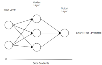
Neural networks are mathematical models inspired by the human brain. It is composed of interconnected neurons arranged in layers. They are trained on data to learn patterns and relationships, enabling tasks such as image recognition, language processing, and decision-making. Neural networks consist of an input layer, hidden layers for processing, and an output layer for generating predictions. Through a process called backpropagation, they adjust their parameters to minimize errors and improve performance during training.

why they are better than classical algorithms:

Neural networks often outperform classical machine learning algorithms in tasks involving complex patterns or large datasets due to their ability to automatically learn hierarchical representations. Unlike classical algorithms that rely on handcrafted features, neural networks can discover and adapt features from raw data. Their capacity for non-linear mapping allows them to capture intricate relationships, making them suitable for tasks like image and speech recognition.

The choice between deep learning and classical machine learning (ML) depends on various factors.

data: Deep learning models often require large amounts of labeled data to generalize well. Classical ML models can perform well with smaller datasets.

Feature Extraction: Deep learning models can automatically learn relevant features from raw data, eliminating the need for manual feature engineering. In scenarios where domain knowledge plays a crucial role, classical ML models may be preferred. They allow for explicit feature engineering.

Computational Resources: Deep learning models, especially large neural networks, require significant computational resources (e.g., GPUs or TPUs) to train efficiently. Classical ML models are often more lightweight and can be trained on less powerful hardware.

Basic Concepts / Building blocks:

Backpropagation:

Backpropagation is a supervised learning algorithm used to train neural networks. It involves two main phases: forward pass and backward pass. In the forward pass, input data is fed through the network to generate predictions. The backward pass then computes the gradient of the loss function with respect to the network’s weights, allowing adjustments to minimize errors. This iterative process of updating weights based on gradients is repeated until the model converges to an optimal configuration, improving its ability to make accurate predictions.

Convergence Criteria

For the model to converge to the dataset, it must reach the global minimum. Initially the parameters of the model will be random, as the model progresses its training it will adjust its parameters such that in next iteration loss values will be reduces, in this process the parameters get tweaked to reach the global minimum.

Wnew = Wold — lr*dL/dw is the formula used for updating the parameters of the model.

Wnew: updated weight

Wold: Old weight

Lr: Learning rate.

dL/dw: Derivative of loss function w.r.t that weight.

Activation Functions:

Activation functions introduce non-linearity to neural networks, enabling them to learn complex patterns.

Sigmoid:

The sigmoid function, also known as the logistic function, is a commonly used activation function in neural networks, especially in the context of binary classification problems. It squashes its input into the range between 0 and 1, which is useful for generating probabilities.

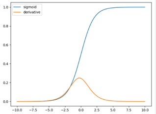
  S(z)=1/(1+e−z) 

Limitations: 

Vanishing Gradient: During backpropagation, gradients can become very small, leading to the vanishing gradient problem. This can result in slow or stalled learning in deep networks.

Computation: Since sigmoid contains exponential in equation computation is expensive.

Output Range: The output of the sigmoid function is not centered around zero, making it less suitable for the optimization of certain network architectures.

Tanh

The hyperbolic tangent function, often abbreviated as tanh, is another commonly used activation function in neural networks. It is similar to the sigmoid function but has a range between -1 and 1. The tanh function squashes its input into the range [−1,1], making it zero-centered. 

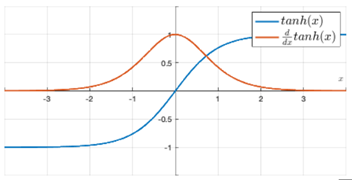
tanh(z)= (ez + e−z) / (ez − e−z)

Limitations of Tanh activation functions:

Vanishing Gradient:

Like the sigmoid function, tanh squashes input values to the range [-1, 1]. This can lead to the vanishing gradient problem during backpropagation, especially in deep networks. The gradients can become very small, causing slow or stalled learning as weight updates become negligible.

Computational Cost:

The tanh function involves exponentiation, which can be computationally more expensive compared to activation functions that only involve simple operations like ReLU. This may impact the overall efficiency of training large neural networks.

RELU

Rectified Linear Unit (ReLU) is a popular activation function used in neural networks. The function is defined as follows: ReLU(z)=max (0, z). In other words, for any given input z, the ReLU function outputs z if z is positive, and 0 otherwise.

RELU and its Derivative 

Advantages of using RELU over Sigmoid and Tanh as activation function.

Non-Saturation:

One of the main advantages of ReLU is that it does not saturate for positive input values. Unlike sigmoid and tanh, where the gradients become very small for extreme values, ReLU maintains a constant positive gradient for positive inputs. This mitigates the vanishing gradient problem, promoting faster and more effective learning.

 Computationally Efficient: 

The ReLU function is computationally efficient to compute compared to sigmoid and tanh, as it involves simple thresholding. The absence of complex mathematical operations like exponentiation makes ReLU faster to compute, leading to quicker training times, especially in deep networks.

Simple and Intuitive:

ReLU is a simple and intuitive activation function. It does not involve complex mathematical operations, making it easy to implement and understand. Its simplicity makes it a popular choice in the design of deep neural networks.

Empirical Success:

ReLU has been widely used in practice and has shown empirical success in various applications, including image classification, natural language processing, and computer vision. Its effectiveness in training deep networks has contributed to its popularity.

Limitations of RELU:

Dead Neurons:

ReLU can suffer from the “dead neurons” problem, where neurons can become inactive during training. If the weighted sum of the inputs to a ReLU unit is consistently negative, the unit’s output will always be zero, and the gradients during backpropagation will be zero. This can prevent the weights of that unit from being updated, causing it to remain inactive.

Exploding Gradients: 

ReLU does not have an upper bound on the activation, and it allows unbounded activation values. This lack of an upper bound can lead to exploding gradients during training, especially in deep networks. Exploding gradients can cause numerical instability and make training difficult.

Lack of Smoothness:

ReLU is not a smooth function because it introduces a sharp bend at zero. This lack of smoothness can make optimization challenging, especially for certain optimization algorithms that rely on smooth gradients.

Optimizers:

Optimizers adjust the model’s parameters during training to minimize the error or loss function. They play a crucial role in the iterative optimization process.

There are many different optimizers, the common ones are:

Gradient Descent (GD): This is the basic optimization algorithm where the model parameters are updated in the opposite direction of the gradient of the loss function with respect to the parameters. It can be slow, especially for large datasets, but it forms the basis for more advanced optimizers.

Formula: W_new = W_old — l_r * ∇f(W_old)

Here we get the derivative of the loss function by considering the whole dataset, thus even though the updating happens in right direction the time taken is very high.

Stochastic Gradient Descent (SGD): In SGD, instead of computing the gradient using the entire dataset, it is computed using only a small subset (mini batch) of the data at each iteration. This can speed up the training process and make it more feasible for large datasets.

Formula: W_new = W_old — l_r * ∇f^(W_old)

The only difference between gradient descent and stochastic gradient descent is instead of considering complete dataset to get derivative of loss function, we consider only sample of data with random selection. Even though the number of steps taken for convergence is high overall time taken will be less compared to Gradient descent.

RMS (Root Mean Square Propagation) Prop: RMSprop is an optimization algorithm commonly used for training neural networks. It is designed to address some of the limitations of other optimization algorithms like stochastic gradient descent (SGD). RMSprop adjusts the learning rates of each parameter individually based on their historical gradients, which can help accelerate convergence.

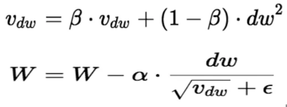
Squared Gradients: RMSprop keeps track of the exponentially decaying average of squared gradients. This is done to normalize the learning rates for each parameter.

Update Rule: The update rule involves dividing the gradient of the current iteration by the square root of the mean of the squared gradients. This helps to scale the learning rates differently for each parameter.

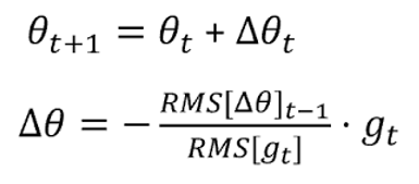
Adadelta: Adadelta is an extension of Adagrad that seeks to address its tendency to decrease the learning rates too aggressively. It uses a running average of squared parameter updates to normalize the learning rates.

Here Learning rate is adapted based on the gradients, if the gradients is high then l_r is also high and vice versa. This will stop the need for manually tuning the learning rate.

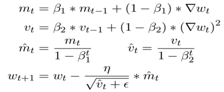
Adam (Adaptive Moment Estimation): Adam is an adaptive optimization algorithm that maintains two moving averages for each parameter — the gradient (first moment) and the squared gradient (second moment). It adapts the learning rates for each parameter based on their past gradients. Adam is widely used in practice and often provides good results with default hyperparameters.

loss functions:

Loss functions measure the difference between the predicted output of a model and the actual target values. They quantify how well or poorly a model is performing. The goal during training is to minimize this loss, guiding the model to make more accurate predictions.

Binary Cross entropy (Logistic Loss):

Used for binary classification problems.

L (y, y^) = -(y*log(y^) + (1-y) *log(1-y^))

y is the true label (0 or 1)

y^ is the predicted probability.

Categorical Cross entropy (SoftMax Loss):

Used for multi-class classification problems. Assumes that each instance can belong to only one class.

L (y, y^) = — sum (yi * log(y^i))

y is the true label (0 or 1)

y^ is the predicted probability.

Sparse Categorical Cross Entropy:

Used for multi-class classification problems. Assumes that each instance can belong to only one class.

Main difference between Categorical Cross entropy and Sparse Categorical Cross Entropy lies in Target label, in case of Categorical Cross entropy target labels are one hot encoded where as in case of sparse Categorical Cross Entropy target labels are integers, each representing the class index.

Ex:

Sparse Categorical Cross entropy: Target=2

Categorical Cross entropy: Target = [0, 0, 1] (one-hot encoded representation indicating class 2)

Mean Squared Error (MSE) / L2 Loss:

Commonly used for regression tasks.

L (y, y^) = 1/n sum (yi — y^i) **2

y is the true label (0 or 1)

y^ is the predicted probability.

Different Types of Neural Network

Briefly Explaining how to fit neural networks for different types of data.

Based on different data types we are working with, there are different neural network architectures. But the Core of Training that is using backpropagation remains the same.

Artificial Neural Network (ANN):

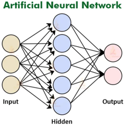
ANNs are the fundamental building blocks of deep learning. They consist of interconnected nodes organized into layers, including an input layer, one or more hidden layers, and an output layer. Each connection between nodes has an associated weight, and the network learns by adjusting these weights during training.

Limitations: ANNs may struggle with processing sequential data and capturing spatial relationships in images effectively.

Convolutional Neural Network (CNN):

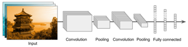
CNNs (Convolutional Neural Network) are widely used in image classification, object detection, and image segmentation tasks. They use convolutional layers to scan input data using filters, enabling the network to automatically learn hierarchical features.

Limitations: CNNs may not perform as well on tasks that involve sequential data.

Recurrent Neural Network (RNN):

RNNs are designed for sequential data processing, making them suitable for tasks like natural language processing and time series analysis. RNNs have recurrent connections that allow them to maintain a hidden state, capturing information from previous inputs in the sequence.

Limitations: Traditional RNNs can struggle with capturing long-range dependencies due to vanishing or exploding gradient problems. They are also computationally intensive and may not scale well for longer sequences.

Long Short-Term Memory with Convolutional layers (LRCN):

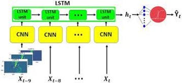
LRCN combines the strengths of CNNs and RNNs. It incorporates convolutional layers to capture spatial features and Long Short-Term Memory (LSTM) cells to model temporal dependencies in sequential data. LRCN is often used for video analysis and action recognition.

Limitations: LRCN models can be computationally expensive and may require significant resources. Training such models also requires a substantial amount of labeled data.

Training / Fitting a Model:

Best Practices on Training the model:

1. Before trying to fit the entire training data, try overfitting only a sample of dataset and see if the model can do it.

2. Make the model overfit the data then work on reducing the complexity of the model.

3. Choose the basic default parameters and try fitting the model, this will give the baseline on which we can choose other parameters to finetune and improve on.

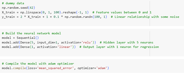
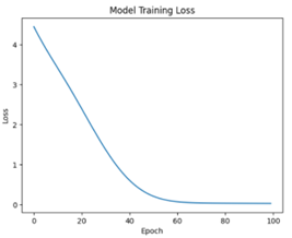
Collab Link: jupyter notebook for training a simple neural network.

AUTHOR - FOLLOW
Jagadeesha R G
Data Scientist Consultant

Detailed Case Study

Enabled Data-Ops on Cloud for a North American Telecom Giant

Learn how a Tredence client integrated all its data into a single data lake with our 4-phase migration approach, saving $50K/month! Reach out to us to know more.

Detailed Case Study

MIGRATING LEGACY APPLICATIONS TO A MODERN SUPPLY CHAIN PLATFORM FOR A LEADING $15 BILLION WATER, SANITATION, AND INFECTION PREVENTION SOLUTIONS PROVIDER

Learn how a Tredence client integrated all its data into a single data lake with our 4-phase migration approach, saving $50K/month! Reach out to us to know more.