Videos and images have become one of the most interesting data sets for artificial intelligence. Camera and imaging hardware being very common. Computer vision enables computers and systems to derive meaningful information from digital images, videos, and other visual inputs — and take actions or make recommendations based on that information. If AI enables computers to think, computer vision enables them to see, observe and understand.

Convolutional Neural Networks

Dense neural networks are universal learners; given a sufficiently large neural network, data of any complexity can be trained and fitted well. With that in mind we can directly have images passed through neural networks and hope that the model picks on the different relations between pixels across channels and classify appropriately. This, however, is a very expensive approach as the number parameters grow high very quickly.

We typically add convolutional layers to help us with reducing dimensions and retaining useful element of the image. Convolution Layers are also easily parallelized on GPUs. They have sensible inductive biases which work well with image data.

A Convolutional neural network (CNN) is a neural network that has one or more convolutional layers and are used mainly for image processing, classification, segmentation and also for other auto correlated data.

A convolution is essentially sliding a filter over the input. A convolution can be thought as looking at a function’s surroundings to make better/accurate predictions of its outcome. Rather than looking at an entire image at once to find certain features it can be more effective to look at smaller portions of the image. Some properties of convolutional operations are:

- Translational Invariance: The features extracted from the convolutional layer are not sensitive to any particular region

- Locality Sensitive: Each convolutional operation takes place in a local region of the image/feature-map and extracts information from the local region in isolation

Convolutional Layers are used in sequence with Pooling Layers. These Pooling Layers help reduce the dimensions of the feature map produced by trying to retain important information and discarding the rest. While this is a lossy process, the benefits gained through speed-up in training and inference are immense.

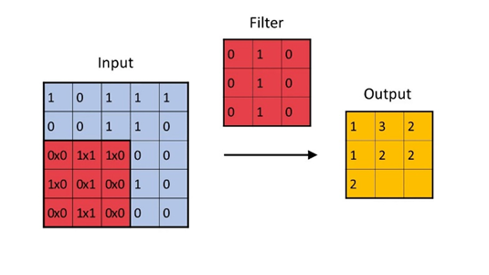
Convolutional Filters in Action

Convolutional filters are the building blocks of the Convolutional Neural Networks. The kernel(s) has a fixed size and is of a square shape (typically a 3x3 or 5x5 matrix). Each of these filters/kernels are supposed to extract some form of information and filter out the rest.

The convolutional operation involves sliding the filters over the image in a systematic way (using stride). The convolution operation can be thought of in the following steps:

1. Superimpose the filter on a local section of Input Image

2. We multiply, element-wise, each cell of the superimposed part of the image with the corresponding cell of filter that is superimposing it.

3. Add all these multiplied values into a single number and place in the output grid

4. Shift the filter and repeat from step 1

5. Repeat this operation across all channels and add across the channel

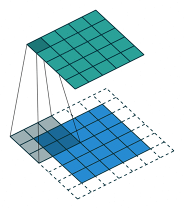
2D Convolution

This way we should cover the image and produce a fresh feature-map. This feature-map is supposed to represent the presence of specific patterns or features in the input image. Filters present in the earlier layers of the convolutional networks can be thought of extracting primitive features such as diagonals edges, crosses etc which the feature-map outputted by these layers show, higher layers can be thought of extracting more complex features and operating on a more sophisticated ontology such as eyes, ears, wheels etc.

There are several parameters involved in working with a convolutional layer

• Filter size: Convolutional Filter is a square matrix, typically of shape 3x3 or 5x5
• Number of Filters/Depth: Each layer of the convolutional layer can have multiple filters. Each filter trying to capture a different feature from the input data
• Stride: Stride determines by how many pixels should the filter move across the image after each operation. A stride of 2 means that the filter skips a pixel by moving 2 pixels over. This can be useful to reduce the dimensions of the output feature-map
• Padding: During convolution, the edge and corner pixels are not covered fully by the filter, only a section of the filter manages to reach these pixels. To increase the coverage, we introduce more pixels around the image, usually using 0s (Zero Padding).

With different parameters we can expect to see changes in the output feature-map’s dimensions.

The output dimension (O) of the feature-map is given by the following:

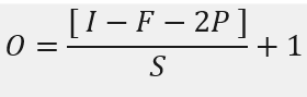
I -> Input image size

F -> Filter shape

P -> Padding

S -> Stride

D -> Depth/Number of Filters

The final shape of the Feature Map is O x D

Pooling Layer

Convolutional Layers, while extracting features, are expected to reduce the dimensionality of the data and retaining the useful parts of the image. Pooling Layers help with reducing the dimensions of the image. Generally, pooling layers are added after the convolutional operation. Pooling operation, like convolution, moves across the feature map with a stride and shape. However, in the pooling layer there is no `depth` and the pooling operation aggregates without any weights or tunable parameters.

Two popular types of Pooling layers available are:

1. Max-Pooling: The maximum value in that local region is picked. A lot of information is lost but this operation is faster compared to average pooling and is generally used in classification and object-detection type tasks

2. Average Pooling: The average of all the values is calculated. This is not as lossy as compared to Max-Pooling due to which it is favoured in more generative approaches; GANs, Auto-Encoders etc.

The output of the pooling layer can be calculated using the same formula as that of the convolutional layer with a few exceptions like the output depth is equal to the input depth. With the pooling layer the stride is generally equal to the pool size.

Receptive Field

With convolutional models, as with all machine learning, we are also interested in understanding the effect of change in input values over the output values. We can measure the influence by checking the receptive field.

The receptive field of a pixel in the k-th layer is denoted by RkxRk of the input that each pixel of the k-th activation map can ‘see’ i.e. changes in those pixels of the input layers will directly influence the activation of our pixel in the k-th layer. Fj (Filter size for layer j) and Si (Stride at layer i) and with the convention S0 = 1, the receptive field of the layer k can be computed with the formula:

Disadvantages and Vulnerabilities of CNN

Adversarial Attacks[3]

By superimposing carefully crafted noise-alike images onto our input image we can easily throw-off our model’s predictions in a completely wrong direction. The superimposed image, to a human eye, still looks perfectly normal and containing the original elements, however, it manages to confuse the model and change its predictions completely.

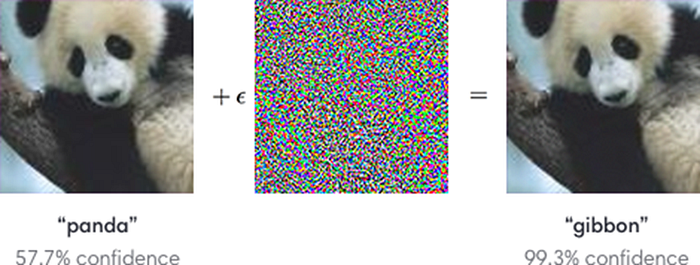
These attacks have been exploited to circumvent surveillance measures taken for security. Wearing a shirt with a distinct pattern on it could deceive object-detection models from detecting the person wearing it[4]

Limited Ability to Generalize

When training CNN models on a set of images, their ontology and colour histogram might be unique to the dataset. If a model is trained on the ImageNet dataset which contains images in well-lit outdoor and indoor environments, it will be sub-optimal to apply the same model towards X-Ray images which have a drastically different colour palette and different objects.

The convolutional operation is a good technique for feature extraction even with randomly initialized filters’ weights [2], however, it is always necessary to re-train the filters as well when the image belong to a completely different class of images with different ontologies and distributions.

Inductive Bias and Lack of Global Understanding

Convolutional operation has a suitable inductive bias when extracting information from images[6]. They offer several desirable properties such as translational invariance and are locality sensitive.

Convolutional, however, lack a global understanding of the image. They extract information well from different parts of the image but cannot model the dependencies between them.

Transformers

Transformers have turned-out to be the de-facto standard for NLP applications. There has also been a steady growth in literature to apply transformers for vision applications. These works have already shown promising results in multiple Computer Vision benchmarks in fields such as Object Detection, Video Classification, Image Classification and Image Generation.

It has been shown that self-attention, in early stages on the model, can learn to behave like a convolution. Transformers do not naturally impose any of the inductive biases seen in convolution. They however can learn these biases.

Some important papers that use transformers for Computer Vision Tasks

- Image Transformer

- ViT (Vision Transformer)

- DETR (Detection Transformer)

Types of Computer Vision Problems

Image Classification

Image classification is a fundamental task in computer vision that involves assigning a label or category to an input image. Over the years, various models and architectures have been developed to improve the accuracy and efficiency of image classification

Some notable Image Classification models over the year are:

1. LeNet: one of the earliest convolutional neural networks (CNNs) designed for handwritten digit recognition. It consists of convolutional layers followed by fully connected layers.
2. AlexNet: a breakthrough model that won the ImageNet Large Scale Visual Recognition Challenge (ILSVRC) in 2012. It popularized the use of deep convolutional neural networks for image classification, with innovations such as the ReLU activation function and the extensive use of data augmentation.
3. VGGNet: The VGGNet architecture, with its simplicity and uniformity, consists of deep networks with small 3x3 convolutional filters. It showed that increasing network depth (number of layers) improves performance.
4. GoogLeNet (Inception v1): the inception module, which uses multiple filter sizes within the same layer and parallel paths for feature extraction. This model emphasized computational efficiency and achieved competitive accuracy with lower computational cost.
5. ResNet (Residual Network): It introduced residual learning, where shortcut connections (skip connections) are used to skip one or more layers. This helps in training very deep networks by mitigating the vanishing gradient problem.
6. DenseNet: DenseNet connects each layer to every other layer in a feedforward fashion. It promotes feature reuse and reduces the number of parameters, leading to improved parameter efficiency.
7. MobileNet: It is designed for mobile and edge devices with limited computational resources. It uses depthwise separable convolutions to reduce the number of parameters and computations while maintaining accuracy.
8. EfficientNet: This algorithm focuses on balancing model depth, width, and resolution to achieve optimal performance. It uses a compound scaling method to scale up or down the model size based on the available resources.
9. ViT (Vision Transformer): ViT represents a departure from traditional CNNs by utilizing transformer architecture for image classification. It divides an image into fixed-size patches, linearly embeds them, and processes them using transformer blocks.

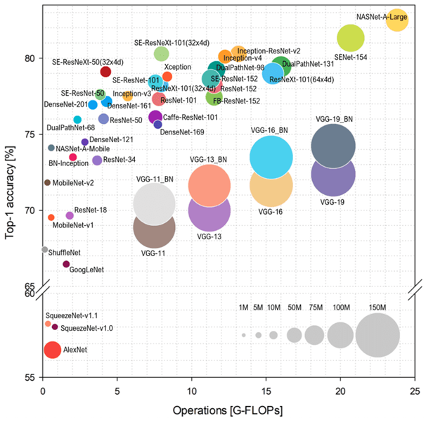
Computational Requirement vs Performance

Object Detection

The goal of object detection is to find what object is where? Usually using a bounding-box, object detection algorithms detect and classify regions of the image.

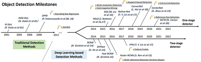
Several datasets have been curated which serve as good training input to the models as well as benchmarks. Some of the most cited and commonly used datasets as benchmarks are the following:

• COCO (Common Objects in Context) Dataset: COCO is a widely used dataset for object detection, segmentation, and captioning. It contains many images with complex scenes and diverse object categories.
• PASCAL VOC (Visual Object Classes): The PASCAL VOC dataset consists of images with 20 object categories, and it is commonly used for benchmarking object detection algorithms. It includes annotations for object bounding boxes.

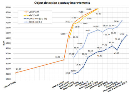
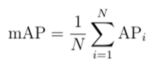
In recent years, the most frequently used evaluation for detection is “Average Precision (AP)”, which was originally introduced in VOC2007. The mean AP (mAP) averaged over all categories is usually used as the final metric of performance.

To measure the object localization accuracy, the IoU between the predicted box and the ground truth is. It is defined through the following formula:

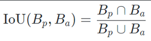
IoU; Where, Bp: Predicted Area, Ba: Actual Area 

Reference

1. Image Benchmark (2011): German Traffic Sign Benchmarks (rub.de)

2. Effectiveness of randomly weighted CNNs: [1802.00844] Intriguing Properties of Randomly Weighted Networks: Generalizing While Learning Next to Nothing (arxiv.org)

3. Adversarial Attacks: Attacking machine learning with adversarial examples (openai.com)

4. Adversarial Attack T-Shirt: [1910.11099] Adversarial T-shirt! Evading Person Detectors in A Physical World (arxiv.org)

5. Object Detection Survey: [1905.05055] Object Detection in 20 Years: A Survey (arxiv.org)

6. Random CNN: 2106.09259.pdf (arxiv.org)

7. Image Transformer: Image Transformer (arxiv.org)

9. Transformers behaving as convolution: 1911.03584.pdf (arxiv.org)`

AUTHOR - FOLLOW
Amey Patil
Data Scientist Consultant

Detailed Case Study

Enabled Data-Ops on Cloud for a North American Telecom Giant

Learn how a Tredence client integrated all its data into a single data lake with our 4-phase migration approach, saving $50K/month! Reach out to us to know more.

Detailed Case Study

MIGRATING LEGACY APPLICATIONS TO A MODERN SUPPLY CHAIN PLATFORM FOR A LEADING $15 BILLION WATER, SANITATION, AND INFECTION PREVENTION SOLUTIONS PROVIDER

Learn how a Tredence client integrated all its data into a single data lake with our 4-phase migration approach, saving $50K/month! Reach out to us to know more.