Part 1: Mastering Image Denoising: Techniques, Challenges, and Solutions

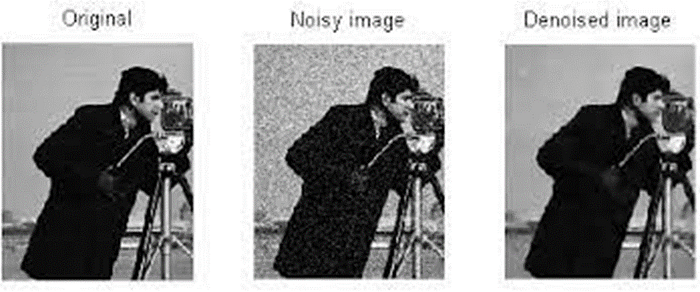
Images captured in real world are subjected to noise due to environment, signal instability, camera sensor issues, poor lighting conditions, electrical loss etc. For further processing these images and to interpret results it is essential to have images with noise as low as possible.

Image Denoising is a critical process in digital image processing, aiming to enhance the visual quality of images by reducing noise. It is challenging topic of active research, involved in understanding the type of noise in the image and thereby apply a denoising method that can reduce the noise and provide more accurate representation of the original image.

Image Denoising as Mathematical Representation

Images with Noise can be represented mathematically as sum of original image with noise.

Observed Image (y) = Unknown Original Image (x) + Gaussian Noise (n)

The main purpose of noise reduction is to decrease the noise in Unknown Original Image while minimizing the loss of the features in the original image and improve the Signal to Noise Ratio.

Challenges:

Challenges in denoising are to smoothen the flat areas while protecting the edges without blurs without generating new objects in the image and maintaining the texture.

From the above mathematical representation, it is not possible to get a unique solution of the original image, we can only get a good estimate of the image.

In this blog, we will look into Classical approaches of Image Denoising and advanced methods using CNN, Auto-Encoders to solve this problem for a simple medical image dataset — Link.

Exploring Various Types of Noise in Images

Images serve as powerful tools for communication, analysis, and interpretation across multiple domains. However, their fidelity can be compromised due to various types of noise, affecting their quality and interpretability. Let’s delve into the distinct types of noise that commonly plague images:'

import cv2
import numpy as np
import matplotlib.pyplot as plt
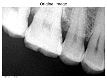
# Load an image
image = cv2.imread('Dataset/1.jpg') # Replace 'path_to_your_image.jpg' with your image path
plt.figure(figsize=(6, 6))
plt.imshow(cv2.cvtColor(image, cv2.COLOR_BGR2RGB))
plt.title("Original Image")
plt.axis('off')
plt.show()

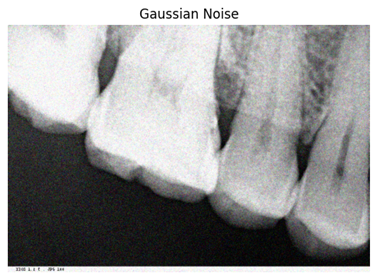
1. Gaussian Noise

Gaussian noise emerges from random variations following a Gaussian distribution. It appears as a subtle, uniform noise that can be introduced during the image acquisition process. Typically, it blurs edges, reduces image clarity, and stems from sources like electronic sensors or transmission errors.

# Function to add Gaussian noise to the image
def add_gaussian_noise(image):
mean = 0
std_dev = 25
h, w, c = image.shape
gaussian = np.random.normal(mean, std_dev, (h, w, c))
noisy_image = np.clip(image + gaussian, 0, 255).astype(np.uint8)
return noisy_image, 'Gaussian Noise'

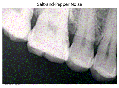
2. Salt-and-Pepper Noise

This type of noise manifests as isolated white and black pixels scattered across an image, akin to grains of salt and pepper. These random pixels are often a result of errors in data transmission or storage. Salt-and-pepper noise can obscure fine details and significantly impact visual interpretation.

# Function to add salt-and-pepper noise to the image
def add_salt_and_pepper_noise(image, amount=0.05):
noisy_image = np.copy(image)
num_salt = np.ceil(amount * image.size * 0.5)
salt_coords = [np.random.randint(0, i-1, int(num_salt)) for i in image.shape]
noisy_image[salt_coords] = 255

num_pepper = np.ceil(amount * image.size * 0.5)
pepper_coords = [np.random.randint(0, i-1, int(num_pepper)) for i in image.shape]
noisy_image[pepper_coords] = 0
return noisy_image, 'Salt-and-Pepper Noise'

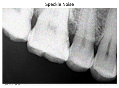
3. Speckle Noise

Speckle noise, prevalent in images acquired through ultrasound or synthetic aperture radar, causes random brightness or darkness variations. It blurs fine details, altering pixel intensities and presenting challenges for image analysis and interpretation.

# Function to add speckle noise to the image
def add_speckle_noise(image):
h, w, c = image.shape
speckle = np.random.randn(h, w, c)
noisy_image = np.clip(image + image * speckle * 0.1, 0, 255).astype(np.uint8)
return noisy_image, 'Speckle Noise'

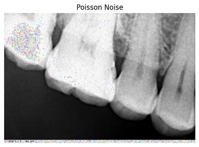
4. Poisson Noise

Arising from the Poisson distribution, this noise is common in low-light photography or astronomical imaging. It appears as grainy artifacts and reduces image contrast and clarity in conditions with minimal light, affecting overall image quality.

# Function to add Poisson noise to the image
def add_poisson_noise(image):
vals = len(np.unique(image))
vals = 2 ** np.ceil(np.log2(vals))
noisy_image = np.random.poisson(image * vals) / float(vals)
return noisy_image.astype(np.uint8), 'Poisson Noise'

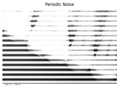
5. Periodic or Banding Noise:

Periodic noise presents as regular patterns or bands across an image, often due to interference or sensor issues. It distorts fine details, altering the image’s appearance and posing challenges for accurate interpretation.

# Function to add periodic or banding noise to the image
def add_periodic_noise(image, frequency=16):
h, w, c = image.shape
x = np.arange(w)
y = np.arange(h)
X, Y = np.meshgrid(x, y)
noise = np.sin(2 * np.pi * frequency * Y / h) * 128 + 128
noisy_image = np.clip(image + noise[..., np.newaxis], 0, 255).astype(np.uint8)
return noisy_image, 'Periodic Noise'

Understanding these various types of noise is crucial for image processing and analysis. Each type exhibits distinct characteristics that impact image fidelity differently, motivating the development of robust denoising techniques.

By comprehensively recognizing these noise variations, researchers and practitioners in image processing aim to devise effective denoising strategies. Advanced techniques, including machine learning-driven approaches like autoencoders, strive to mitigate these noise influences, restoring image quality and enabling accurate analysis across diverse applications.

Classical Approach for Image Denoising

Spatial domain filtering:

Spatial domain filtering involves manipulating an image’s pixel values directly in the spatial domain (the image itself) to enhance or modify its characteristics. Different filter types are used in spatial domain filtering to achieve various effects:

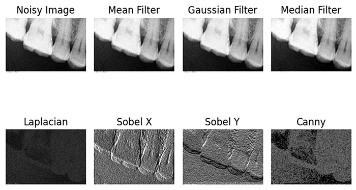
1. Smoothing Filters:

Mean Filter: Replaces each pixel’s value with the average of its neighboring pixels. It reduces noise but may blur edges and fine details.

Gaussian Filter: Assigns weights to neighboring pixels based on a Gaussian distribution. It smoothens the image while preserving edges better than mean filtering.

2. Sharpening Filters:

Laplacian Filter: Enhances edges by highlighting sudden intensity changes. It emphasizes edges but also amplifies noise.

High-pass Filter: Emphasizes high-frequency components, making edges and details more pronounced. It can enhance images but may also amplify noise.

3. Edge Detection Filters:

Sobel and Prewitt Filters: Identify edges by calculating gradients in horizontal and vertical directions. They highlight edges with different orientations.

Canny Edge Detector: More advanced, it uses multiple steps to detect edges accurately by suppressing noise and finding local maxima in gradients.

4. Other Filters:

Median Filter: Replaces a pixel’s value with the median of neighboring pixels. Effective in removing salt-and-pepper noise while preserving edges.

Bilateral Filter: Retains edges while reducing noise. It smoothens images based on both spatial and intensity differences.

Spatial Domain Filtering Process:

Convolution Operation: Filters are applied through convolution, where a filter kernel moves over the image, computing new pixel values based on weighted sums of neighboring pixels.

Filter Size and Parameters: The size and values of the filter kernel (mask) determine the effect of the filter on the image. Larger kernels have a more extensive smoothing effect, but they can blur details.

Considerations:

Computational Complexity: Some filters require more computational resources due to larger kernel sizes or complex operations.

Edge Preservation: Smoothing filters can blur edges, impacting the overall sharpness of the image.

Artifact Reduction: Filters like median and bilateral can effectively reduce specific types of noise while preserving image details.

Application:

Spatial domain filtering finds applications in image denoising, edge detection, image enhancement, and feature extraction across various fields like medical imaging, computer vision, and photography.

Understanding these filter types helps in choosing the appropriate filter for a specific image processing task based on the desired outcome and the nature of the image and noise.

import cv2
import numpy as np
import matplotlib.pyplot as plt

# Load an image
image = cv2.imread('Dataset/1.jpg', 0)  # Replace 'path_to_your_image.jpg' with your image path and load as grayscale

# Add noise to the image (example: Gaussian noise)
def add_gaussian_noise(image):
    mean = 0
    std_dev = 25
    h, w = image.shape
    gaussian = np.random.normal(mean, std_dev, (h, w))
    noisy_image = np.clip(image + gaussian, 0, 255).astype(np.uint8)
    return noisy_image

noisy_image = add_gaussian_noise(image)

# Apply different filters to the noisy image
filtered_mean = cv2.blur(noisy_image, (5, 5))  # Mean filter (5x5 kernel)
filtered_gaussian = cv2.GaussianBlur(noisy_image, (5, 5), 0)  # Gaussian filter (5x5 kernel)
filtered_median = cv2.medianBlur(noisy_image, 5)  # Median filter (5x5 kernel)
laplacian = cv2.Laplacian(noisy_image, cv2.CV_8U)  # Laplacian filter
sobel_x = cv2.Sobel(noisy_image, cv2.CV_8U, 1, 0, ksize=5)  # Sobel X filter (5x5 kernel)
sobel_y = cv2.Sobel(noisy_image, cv2.CV_8U, 0, 1, ksize=5)  # Sobel Y filter (5x5 kernel)
canny = cv2.Canny(noisy_image, 100, 200)  # Canny edge detection

# Display the original noisy image and filtered images
titles = ['Noisy Image', 'Mean Filter', 'Gaussian Filter', 'Median Filter', 'Laplacian', 'Sobel X', 'Sobel Y', 'Canny']
images = [noisy_image, filtered_mean, filtered_gaussian, filtered_median, laplacian, sobel_x, sobel_y, canny]

for i in range(len(images)):
    plt.subplot(2, 4, i + 1)
    plt.imshow(images[i], cmap='gray')  # Display as grayscale
    plt.title(titles[i])
    plt.axis('off')

plt.tight_layout()
plt.show()
 

Variational denoising methods:

Variational denoising methods are a class of image denoising techniques that aim to remove noise from images by minimizing an objective function or energy functional. These methods are grounded in variational principles and often use mathematical models to regularize the image in a way that retains important features while reducing noise. Here’s a detailed breakdown:

1. Variational Denoising Principle:

Energy Functional: Formulates denoising as an optimization problem by defining an energy functional that consists of a data term and a regularization term.

Data Term: Measures the discrepancy between the noisy image and the desired denoised image.

Regularization Term: Encodes prior knowledge about the characteristics of the noise and the desired properties of the denoised image.

2. Variational Models:

Total Variation (TV) regularization

Total Variation (TV) regularization is a technique used in image processing for denoising and image reconstruction. It’s a popular method due to its ability to preserve edges and fine details while effectively reducing noise.

Basics of TV Regularization:

Objective:

The main objective of TV regularization is to minimize the total variation of an image while preserving important structures such as edges.

Total Variation:

In simple terms, the total variation of an image measures the amount of intensity variation present in the image. Mathematically, for a grayscale image 

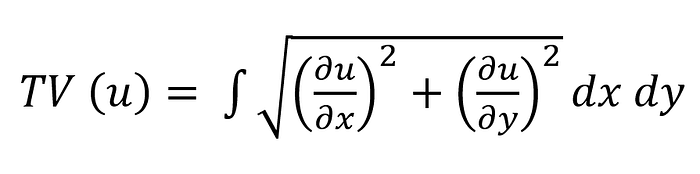
∂u/∂x and ∂u/∂y represent the gradients in the horizontal and vertical directions, respectively.

Denoising with TV Regularization:

When applied to denoising, the TV regularization technique minimizes the total variation of the noisy image while preserving edges. It achieves this by seeking a denoised image that simultaneously maintains smooth regions and sharp transitions (edges).

TV Regularization in Denoising:

· Noise Reduction: TV regularization effectively reduces noise while retaining sharp features like edges and textures. It penalizes high-frequency components in the image that are typically associated with noise.

· Edge Preservation: The key advantage of TV regularization is its ability to preserve edges. As it minimizes the total variation, it favors piecewise smooth regions, effectively preserving edges as areas of high variation.

· Mathematical Optimization: TV-based denoising is formulated as an optimization problem, aiming to find a denoised image that minimizes the total variation while being close to the noisy image. Techniques like gradient descent or more sophisticated optimization algorithms are used to solve this problem iteratively.

Considerations and Challenges:

· Parameter Tuning: TV regularization methods often involve tuning parameters like the regularization parameter (λ) to balance between denoising and preserving image structures.

· Computational Complexity: The optimization involved in TV regularization can be computationally intensive, especially for large images or high-resolution data.

· Artifacts: In some cases, TV denoising might introduce artifacts known as staircase effects, where smoothed regions might appear blocky or exhibit unnatural edges.

Applications:

· Medical Imaging: TV regularization is used in various medical imaging tasks like MRI denoising, CT image reconstruction, etc., to enhance image quality.

· Image Restoration: It’s applied in image restoration tasks to remove noise and enhance image details.

· Computer Vision: TV regularization finds applications in computer vision tasks like object detection, edge detection, and feature extraction due to its edge-preserving properties.

ROF (Rudin-Osher-Fatemi) Model: Uses TV regularization and iteratively solves a convex optimization problem to obtain a denoised image. The ROF model is an optimization-based technique that adds an extra constraint to the TV regularization to enhance denoising capabilities:

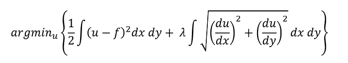
Here:

1. u is the denoised image
2. f is the noisy input image.
3. λ is the regularization parameter balancing the data fidelity term and the total variation term.

Denoising Process in ROF Model:

The ROF model formulates denoising as an optimization problem that seeks a denoised image u by balancing two terms:

· Data Fidelity Term: Minimizes the difference between the denoised image and the noisy image.

· Total Variation Term: Encourages the smoothness of the denoised image while preserving edges by minimizing total variation.

Advantages of ROF Model:

· Improved Denoising: ROF enhances denoising capabilities compared to basic TV regularization by introducing an extra constraint.

· Edge Preservation: It effectively preserves edges and fine details in the image while reducing noise.

· Mathematical Optimization: It utilizes optimization techniques to find the denoised image that minimizes the total variation and fits the noisy input.

Applications:

· Medical Imaging: ROF model finds applications in MRI denoising, CT image reconstruction, and other medical imaging tasks.

· Image Restoration: It’s applied in restoration tasks to remove noise while preserving crucial image structures.

Computer Vision: ROF model is used in computer vision applications involving edge preservation, feature extraction, and object detection.

import cv2
import numpy as np
import matplotlib.pyplot as plt

# Load an image
image = cv2.imread('Dataset/1.jpg', cv2.IMREAD_GRAYSCALE)  # Load as grayscale

# Add Gaussian noise to the image
def add_gaussian_noise(image):
    mean = 0
    std_dev = 1
    noise = np.random.normal(mean, std_dev, image.shape).astype(np.uint8)
    noisy_image = cv2.add(image, noise)
    return noisy_image

noisy_image = add_gaussian_noise(image)

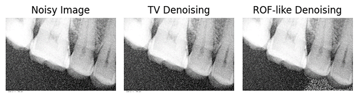
# Total Variation (TV) Denoising
def tv_denoising(image):
    # Ensure the image is float32 for denoising
    image = image.astype(np.float32) / 255.0
    tv_denoised = cv2.denoise_TVL1(image, None, 5)
    if tv_denoised is None:
        return image * 255.0  # If denoising fails, return the original image
    return (tv_denoised * 255.0).astype(np.uint8)

tv_denoised_image = tv_denoising(noisy_image)


# Rudin-Osher-Fatemi (ROF) Denoising
def rof_denoising(image, alpha, lambda_, num_iters):
    u = image.astype(np.float32) / 255.0  # Initial solution
    height, width = u.shape

    for _ in range(num_iters):
        # Compute gradients
        grad_x = np.roll(u, -1, axis=1) - u
        grad_y = np.roll(u, -1, axis=0) - u

        # Update solution using ROF denoising formula
        u += alpha * (lambda_ - np.sqrt(grad_x**2 + grad_y**2))

    return (u * 255.0).astype(np.uint8)

# ROF Denoising parameters
alpha = 0.001 # Regularization parameter
lambda_ = 0.1  # Lambda parameter
num_iters = 30  # Number of iterations

rof_denoised_image = rof_denoising(noisy_image, alpha, lambda_, num_iters)


# Display the original noisy image, TV denoised image, and ROF-like denoised image
titles = ['Noisy Image', 'TV Denoising', 'ROF-like Denoising']
images = [noisy_image, tv_denoised_image, rof_denoised_image]

for i in range(len(images)):
    plt.subplot(1, 3, i + 1)
    plt.imshow(images[i], cmap='gray')
    plt.title(titles[i])
    plt.axis('off')

plt.tight_layout()
plt.show()

import cv2
import numpy as np
import matplotlib.pyplot as plt

# Load an image
image = cv2.imread('Dataset/1.jpg', cv2.IMREAD_GRAYSCALE)  # Load as grayscale

# Add Gaussian noise to the image
def add_gaussian_noise(image):
    mean = 0
    std_dev = 1
    noise = np.random.normal(mean, std_dev, image.shape).astype(np.uint8)
    noisy_image = cv2.add(image, noise)
    return noisy_image

noisy_image = add_gaussian_noise(image)

# Total Variation (TV) Denoising
def tv_denoising(image):
    # Ensure the image is float32 for denoising
    image = image.astype(np.float32) / 255.0
    tv_denoised = cv2.denoise_TVL1(image, None, 5)
    if tv_denoised is None:
        return image * 255.0  # If denoising fails, return the original image
    return (tv_denoised * 255.0).astype(np.uint8)

tv_denoised_image = tv_denoising(noisy_image)


# Rudin-Osher-Fatemi (ROF) Denoising
def rof_denoising(image, alpha, lambda_, num_iters):
    u = image.astype(np.float32) / 255.0  # Initial solution
    height, width = u.shape

    for _ in range(num_iters):
        # Compute gradients
        grad_x = np.roll(u, -1, axis=1) - u
        grad_y = np.roll(u, -1, axis=0) - u

        # Update solution using ROF denoising formula
        u += alpha * (lambda_ - np.sqrt(grad_x**2 + grad_y**2))

    return (u * 255.0).astype(np.uint8)

# ROF Denoising parameters
alpha = 0.001 # Regularization parameter
lambda_ = 0.1  # Lambda parameter
num_iters = 30  # Number of iterations

rof_denoised_image = rof_denoising(noisy_image, alpha, lambda_, num_iters)


# Display the original noisy image, TV denoised image, and ROF-like denoised image
titles = ['Noisy Image', 'TV Denoising', 'ROF-like Denoising']
images = [noisy_image, tv_denoised_image, rof_denoised_image]

for i in range(len(images)):
    plt.subplot(1, 3, i + 1)
    plt.imshow(images[i], cmap='gray')
    plt.title(titles[i])
    plt.axis('off')

plt.tight_layout()
plt.show()
 

Low-rank minimization

Low-rank minimization is a technique used in image processing and computer vision for tasks such as denoising, super-resolution, and image completion. It’s based on the assumption that images or their representations can be approximated by low-rank matrices or tensors.

The primary goal of low-rank minimization is to approximate a given data matrix (image) by a low-rank matrix by minimizing a suitable rank-based regularization term.

Low-rank Matrix:

A matrix is said to be low-rank if it can be well approximated by a matrix of much smaller rank. For an image, this suggests that its information or structure can be efficiently represented using a reduced number of basis elements or features.

Singular Value Decomposition (SVD):

Low-rank minimization often involves decomposing the given matrix using techniques like Singular Value Decomposition. The optimization problem incorporates a low-rank term as a regularization to enforce the solution to have a low-rank representation:

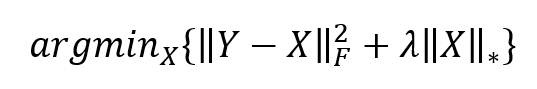
Here:

Denoising with Low-rank Minimization:

Low-rank minimization aims to find a low-rank approximation of a noisy or corrupted image by balancing fidelity to the observed data and the constraint of having a low-rank structure.

Advantages of Low-rank Minimization:

· Noise Reduction: It effectively reduces noise while retaining important features by approximating the image with a low-rank representation.

· Feature Preservation: Low-rank minimization can preserve structures, edges, and important features of an image during denoising or restoration.

· Adaptive Nature: It adapts to various noise levels and image characteristics, making it versatile for different denoising tasks.

Applications:

· Image Denoising: Low-rank minimization is used in denoising tasks, particularly when dealing with noise in images.

· Super-resolution: It’s applied in enhancing image resolution by reconstructing high-resolution images from low-resolution inputs.

· Image Completion: In scenarios where parts of images are missing or corrupted, low-rank minimization can help complete or restore those regions.

Low-rank minimization techniques play a vital role in image processing tasks, offering effective denoising capabilities and preserving crucial features within images. Their ability to reduce noise while maintaining important structures makes them valuable in various domains requiring high-quality image processing.

Along with these methods of variational denoising, there are other methods like Non-Local Regularization, Sparse Representation.

In the next blog, we can see the Transformed domain filtering methods along with CNN denoising.

AUTHOR - FOLLOW
Aravind Madan Mohan
Data Scientist, Tredence Inc.

Detailed Case Study

Enabled Data-Ops on Cloud for a North American Telecom Giant

Learn how a Tredence client integrated all its data into a single data lake with our 4-phase migration approach, saving $50K/month! Reach out to us to know more.

Detailed Case Study

MIGRATING LEGACY APPLICATIONS TO A MODERN SUPPLY CHAIN PLATFORM FOR A LEADING $15 BILLION WATER, SANITATION, AND INFECTION PREVENTION SOLUTIONS PROVIDER

Learn how a Tredence client integrated all its data into a single data lake with our 4-phase migration approach, saving $50K/month! Reach out to us to know more.